Prediction Boundary
Where prediction helps in a delayed optical loop
18 November 2026 · Technical report
Abstract
Adaptive optics corrects light using measurements of a wavefront that has already begun to change. We compare five controllers in a delayed pyramid-sensor simulation, freezing their settings before 600 held-out trials. A two-tap predictor reduced residual wavefront error relative to a tuned integrator in five of twelve conditions, all at the lower photon level. Seven comparisons remained uncertain. A learned mixture did not outperform both of its reference controllers in any condition. We release the complete comparisons, raw evidence, and a notebook that reconstructs the statistical result. The contribution is a reproducible map of where these controllers differ within a specified model; it does not establish instrument performance.
1. A correction arrives in the future
A telescope does not receive a perfectly flat wavefront. Patches of atmosphere delay different parts of the incoming light by different amounts. A deformable mirror can undo some of that distortion, provided the instrument can measure it and act quickly enough.
The difficulty is that “quickly enough” is a moving target. The sensor measures one state of the atmosphere. The mirror applies a correction to a later state. Even an accurate measurement can become the wrong instruction if it arrives late.
A small calculation makes the scale tangible. The simulated timestep is 1 ms and the command delay is two frames. Our first atmospheric layer moves at 10 m/s before the wind multiplier. At the slow and fast settings, it therefore travels
For orientation, the model’s one-metre pupil spans 32 samples: about 31 mm per grid spacing. The fast layer moves roughly one grid spacing while the command waits. This is a geometric estimate, not a measured error budget. It explains why remembering how a wavefront is moving could be useful.
Predictive adaptive optics has a substantial history. Empirical orthogonal-function controllers, for example, learn temporal relationships from wavefront-sensor histories [1]. Here we ask a narrower question: with this sensor, delay, noise model and fixed training budget, where does a simple predictor earn an advantage over a tuned integrator?
2. Five controllers, one frozen comparison
An integrator accumulates corrections from the measured residual. Our baseline is leaky: it retains 99% of the previous issued command and adds half the current reconstructed residual. Before clipping, its modal command is
The predictor first adds the applied mirror command back to the measured residual. This produces a noisy estimate of the incoming wavefront, often called pseudo-open-loop telemetry. For each mode, it combines the current and previous estimates:
The coefficients are fitted on noisy training telemetry, separately for each episode, then averaged with equal episode weight. The predictor receives no future phase or simulator truth as a measurement. Validation selected a one-frame fitting horizon and ridge coefficient 0.01. That fitting horizon is distinct from the physical two-frame command delay, which remains the same for every controller.
| Controller | What changes | Selected setting |
|---|---|---|
| Integrator | Accumulates linearly reconstructed residuals | Gain 0.5; leak 0.99 |
| Predictive | Fits two temporal coefficients per mode | Horizon 1; ridge 0.01 |
| Nonlinear forward | Fits the sensor image through the optical model | Three estimator steps; gain 0.5; leak 0.99 |
| Fixed mixture | Combines linear and forward commands by a fixed rule | Gain 0.5; leak 0.99 |
| Learned mixture | Learns per-mode weights between those commands | 20 Adam steps; gain 0.5; leak 0.99 |
Each family had six candidates and twenty validation trials per candidate. Selection used only clean validation conditions, chose one candidate globally per family, and froze it before evaluation. Equal search opportunity does not mean equal compute or equally expressive algorithms. The learned network had one initialization and a finite optimization budget.
Evaluation crossed two photon levels, two wind speeds and three conditions: clean operation, optical-gain drift, and vibration. Within each condition, the five controllers shared ten atmosphere seeds and detector keys. Their photon observations need not be identical: different commands change the light reaching the sensor.
The simulation uses a 32 × 32 pupil, 100 controlled modes, an unmodulated pyramid wavefront sensor, a 64 × 64 detector, and 750 nm light. Optical-gain drift reduces the sensor response toward 0.35; vibration injects a 0.7 rad, 40 Hz component. These are specified stress cases. They are not a survey of the disturbances an observatory encounters.
3. The advantage has a boundary
Prediction had a supported advantage over the integrator in five of twelve conditions. All five were at 1,000 photons per frame. At 1,000,000 photons, all six comparisons remained uncertain. The remaining low-flux case, slow wind with optical-gain drift, was also uncertain. Only two photon levels were tested; we have not located a flux threshold at which prediction becomes useful.
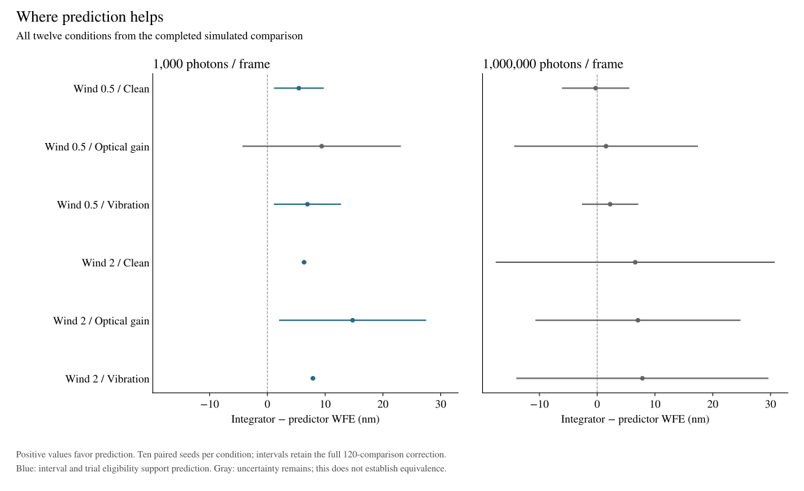
Consider the clean, low-flux, fast-wind condition. Mean residual wavefront error fell from 49.10 to 42.75 nm. The paired difference was 6.35 nm, with a simultaneous interval of [6.07, 6.63] nm. Expressed relative to the integrator’s mean:
This is a ratio of condition means, not a mean of per-seed percentage improvements. It describes one declared condition. It is not a 13% improvement in telescope images, and it is not an average over the whole study.
Both the integrator and the predictor use history. They use it differently. There is a plausible reason for a fitted temporal relationship to matter in a noisy loop: past measurements contain information about the current disturbance, while reacting strongly to a noisy current measurement can inject error. Our experiment does not isolate that mechanism. It changes photon level and wind but does not separately remove the predictor’s temporal filtering and extrapolation. The result is a measured conditional advantage; the explanation remains a hypothesis to test.
The uncertain high-flux comparisons deserve equal attention. An interval crossing zero means the experiment did not resolve the direction of the difference under its reporting rule. It does not establish equality, nor does it prove that prediction stops helping when the sensor gets brighter.
The clean, fast-wind pair is particularly revealing. Its high-flux mean difference is 6.58 nm, close to the low-flux value of 6.35 nm. But one high-flux seed contributes a 46.40 nm difference while the other nine range from about 1.98 to 2.48 nm. The resulting interval is [−17.44, 30.61] nm. The average conceals a very different distribution of evidence.
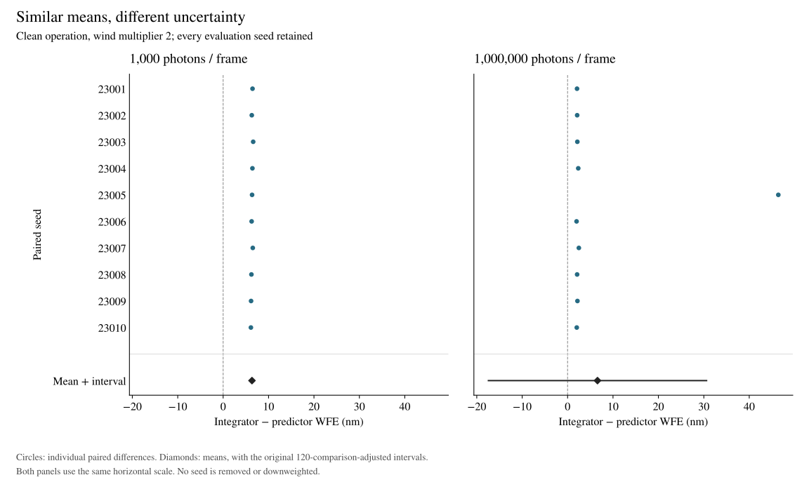
We have not established why that trajectory differs. Removing it because it is inconvenient would change the experiment after seeing the answer. For an instrument, a rare, large discrepancy is often exactly the case worth understanding.
4. What the numbers actually measure
For each trial, we measure the residual phase variance across the pupil after removing piston, a uniform phase offset. Wavefront error converts that phase variance to a length. With wavelength λ and the 384 post-burn-in frames T, the score is
The square root comes after averaging the variances. Averaging framewise RMS values would answer a different question. Each 512-frame episode discards the first 128 frames. Faults begin at frame 256, so the primary score deliberately contains both pre-fault and faulted operation. Fault-window-only comparisons are retained as exploratory results.
Uncertainty is calculated over paired atmosphere seeds, not over thousands of correlated frames. For each condition we form ten differences, ds = WFEintegrator,s − WFEpredictive,s. The reported interval is
There are ten controller pairs in each of twelve conditions: 120 comparisons. Each Student-t interval has exact coverage under independent, normally distributed seed-level differences; Bonferroni then gives at least 95% family coverage. With ten seeds, departures from that model can matter. Correlation between conditions does not itself invalidate Bonferroni.
An interval excluding zero is only part of the decision. Every trial of the proposed winner must also be finite, beat its paired zero-mirror reference, and keep saturation at or below 1% of frames. No minimum practically valuable WFE difference was specified. A statistically separated result can still be too small to matter to an instrument.
5. What the learned controller did not establish
The learned mixture beat the integrator in three conditions and the nonlinear forward controller in five. It beat both in none. The forward controller beat the learned mixture in two conditions. Some learned–forward differences were only hundredths of a nanometre.
That limits the claim we can make about this implementation. It does not settle whether learned control is useful. Training used a small shared weighting network, one initialization, twenty Adam steps and Gaussian pathwise noise; evaluation used Poisson sampling plus read noise. The study does not separate architectural limitations from optimization quality or that training–evaluation mismatch.
The same restraint applies to the successful predictor. It is a per-mode, two-tap model. We did not compare it against a stronger multivariate predictor or a linear–quadratic–Gaussian (LQG) controller. Established predictive-control methods are the relevant next baselines [1], rather than a claim of novelty for prediction itself.
6. From a smaller residual to a better instrument
A controller can improve a wavefront metric without delivering the expected improvement in a science image. The distinction is visible in real work: Fowler and colleagues’ 2026 Keck report describes improved wavefront-sensor residuals while NIRC2 Strehl and coronagraph-free contrast remained comparable between the predictor and integrator [2]. Their on-sky result and our simulation concern different systems; their percentages are not a benchmark for ours.
There is a second distinction between simulated time and execution time. Our loop advances by 1 ms per simulated frame. That does not mean its implementation can read a sensor, calculate a command and update a mirror within 1 ms. The retained acquisition costs include compilation, synchronized execution and evidence writing. They are not a latency distribution or a deadline guarantee.
The next instrument experiment therefore needs three synchronized records: what the sensor observed, what the actuator actually applied, and what happened to science quality. It also needs the calibration in force, the existing controller as a baseline, and event timestamps precise enough to tell which information was available when each command was chosen.
Calibration drift and recovery are separate milestones in our programme. A good predictor does not prove that a detector will notice drift, and a detected problem does not prove that switching controllers will help. Our scheduled-fallback study tests the latter question separately. We will report its complete cohort rather than infer recovery performance from the comparison here.
7. Reproduce the result
The companion notebook downloads the 1.35 MB, checksum-pinned report and reconstructs all 120 primary comparisons from its per-trial metrics. It checks the complete trial identities, pairs seeds, recomputes the intervals and applies the usefulness and saturation requirements. It also recreates Figures 2 and 3 and the 13% calculation. No GPU or model API is needed. Download the notebook to run it locally.
This is a statistical reproduction of published trial metrics. Full physical reproduction is a larger task. The raw release contains 7,228 files and 40.35 GB of sensor, phase, command and training evidence. The download guide pins the dataset revision and verifies its contents.
A separate NumPy audit reconstructed residual variance, coherent pupil Strehl, zero-mirror references, command delay and modal bounds across all 1,200 validation and evaluation trials. It passed the stated absolute-plus-relative tolerances. It uses the saved pupil, basis and atmosphere, so it is not an independent validation of the sensor model. The audit was specified after the main result was observed and before the audit was run.
The original protocol, selection, complete report and physical audit remain available. This completed cohort is exposed. It can support inspection and exploratory analysis; a new confirmatory claim needs new, disjoint evaluation data.
References
- Olivier Guyon and Jared Males. Adaptive Optics Predictive Control with Empirical Orthogonal Functions (EOFs). 2017. arXiv:1707.00570.
- Jules Fowler et al. Ground control to major time-lag: on-sky results of data-driven predictive wavefront control at Keck Observatory. 2026. arXiv:2606.20838.
- Noether Labs. Fair controller-validation protocol v1, and Prediction Boundary retained results. 2026. Source and complete comparison record.
Cite this report
Noether Labs. Prediction Boundary: Where prediction helps in a delayed optical loop. 2026. https://www.noether.one/research/prediction-boundary
@misc{noether2026predictionboundary,
  title = {Prediction Boundary: Where prediction helps in a delayed optical loop},
  author = {{Noether Labs}},
  year = {2026},
  url = {https://www.noether.one/research/prediction-boundary}
}
For research exchange or a recorded calibration-drift problem, write to founders@noether.one.